|
|
|
The 2D-CTTVA method (Blagau et al, 2010) extends the planar timing method (see e.g. Haaland et al., 2004) in order to accommodate situations when the MP behaves like a two-dimensional, non-planar discontinuity . This is the case, for example, when the single-spacecraft technique relying on minimum variance
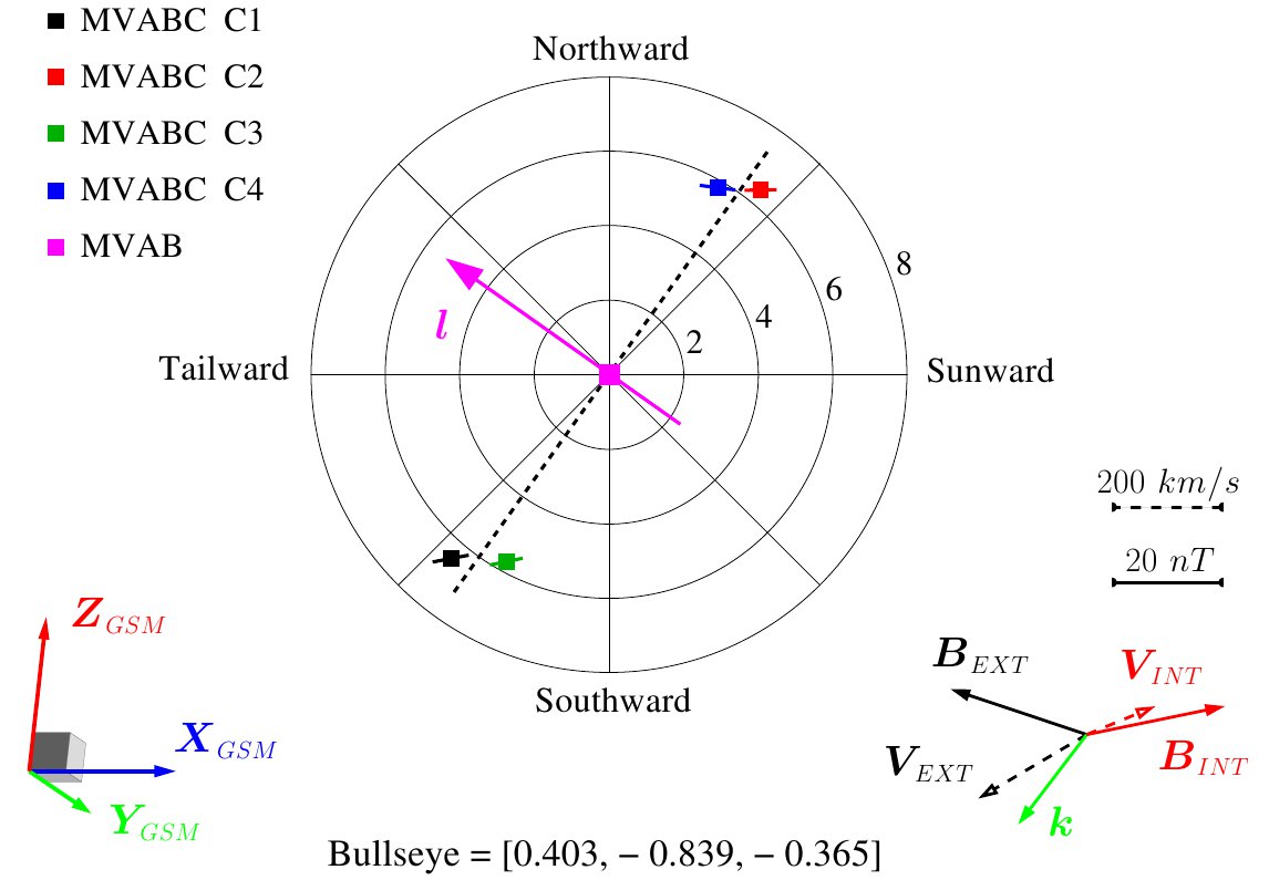
analysis of the magnetic field (MVAB) provides different individual MP normals, all of them contained approximately in the
same plane (see Fig. 1). Such a configuration is not necessarily related to experimental errors, but can have natural causes, like a local bulge/indentation in the MP or a large amplitude traveling wave on this surface. The technique is ilustrated below with a test case.
|
|
In one implementation of the method, the MP is locally modeled as a layer of constant curvature and thickness, oriented along the invariant direction l (introduced in Fig. 1) and moving along two perpendicular directions. Knowing the times when each satellite detects the MP leading and trailing edge, we can solve a system of equations for determining the spatial scale of the structure (radius of curvature and thickness), the direction of movement and its evolution in time, assuming a polynomial dependence for the displacement (a total of 8 model parameters).
|
|
Fig. 1 Polar plot showing the orientation of the four individual normals (MVAB C1-C4) with respect to their average, taken as reference direction in space (symbol MVAB; the circles designate directions of equal inclination, in degrees). The individual normals are located roughly in one plane (dashed line) indicating a two-dimensional MP with the invariant direction oriented perpendicular (unit vector l).
|
|
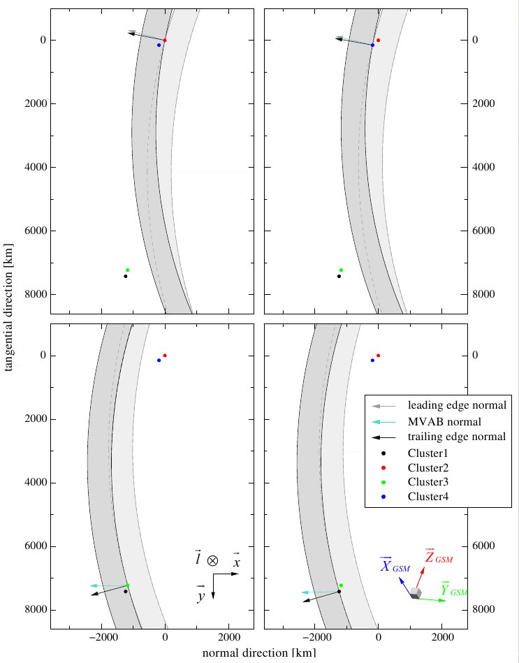
The obtained solution is presented in Fig. 2. In contrast to the planar situation, the instantaneous, non-planar normals at each spacecraft location are linked through the MP geometry and dynamics.
The global (over the 4 satellites) magnetic variance along the instantaneous, 2D MP normals is less than the same quantity computed based on planar results. This is an independent confirmation that, indeed, the model correctly describes the MP behaviour for this event.
|
|
|
|
|
Fig. 2 Graphical representation of the obtained solution. The drawings are MP cuts in a plane perpendicular to the invariant direction l (which is pointing into the page). The satellite positions are indicated by the colored dots and the MP moves along the x axes with constant velocity, whereas along the y axes it has a more complicated, back and forth motion. Each of the four panels is associated with one satellite and shows the MP configuration at two times: when the respective satellite enters the layer (light gray) and when it leaves the layer (darker gray). The MP geometrical normals at the satellite position and for these two times are shown, together with the individual normals obtained from the MVAB technique (green arrows).
|
|
The method was further improved by incorporating in a self-consistent way the requirement of minimum magnetic field variance along the magnetopause normal.
|
|
|
|
|
The movies below present the magnetopuase motion according to two solutions provided by the 2D-CTTVA method. On the right, the MP is locally modelled as a layer of parabolic shape that moves vith constant velocity along the x axes whereas the motion along the y axes is described by a third dedree polinomial. On the left, the MP is locally modelled as a layer of constant curvature that moves vith constant velocity along the y axes whereas the motion along the x axes is described by a third dedree polinomial. In both movies the invariant direction l is out of the screen. The direction of MVAB normals, the evolution of instantaneous normals during the MP crossing and the average crossing parameters are shown on the top.
|
|
|